Graphics with ggplot2
Introduction to ggplot2
R's package ggplot2 is based on a 'grammar of graphics' framework which follows a layered approach to construct graphics in a structured manner. All graphics in this package use layers to create the final graphic. A layer has 5 important components:
Data - the source of the information to be visualized.
ggplot(data=airquality, ...
Mapping - 'aesthetics' how the variables are applied to the graph in terms of X and Y position, stratification, colors etc.
ggplot(data=airquality, mapping = aes(x=Temp)) + ...
Statistical transformation - includes value transformations, calculating means for bar plots, adding a regression line etc. Every geometric object function has a default statistic.
Geometric objects - points, lines, bars, text
... geom_density()
Scales - A scale controls how data interact with aesthetic attributes. Particularly important are the color scales.
... scale_fill_manual(values = c("red", "blue", "green"))
Coordinate system - most often you will likely use the default coordinate system - the Cartesian system.
Visual overview
If you are new to ggplot2, I highly recommend to work through the entire tutorial. If you are just interested in a specific graph, select the desired thumbnail below.


Example data airquality
Data represent daily air quality measurements in New York, May to September 1973. The variables Ozone and Solar.R have several missing values.
| No | Var | Type | Description |
|---|---|---|---|
| 1 | Ozone | number | Ozone (ppb) |
| 2 | Solar.R | number | Solar radiation (lang) |
| 3 | Wind | number | Wind speed (mph) |
| 4 | Temp | number | Temperature (°F) |
| 5 | Month | number | Month (1--12) |
| 6 | Day | number | Day of month (1--31) |
Example data birthwt
This dataset is in the package MASS. The aim of the study was to assess risk factors associated with low infant birth weight collected at a medical center in US during 1986. 189 women were enrolled in the study.
| No | Var | Type | Description |
|---|---|---|---|
| 1 | low | number | Birth weight less than 2.5 kg (0/1) |
| 2 | age | number | Mother's age [years] |
| 3 | lwt | number | Mother's weight at last menstrual period [pounds] |
| 4 | race | number | Mother's race (1 = white, 2 = black, 3 = other) |
| 5 | smoke | number | Smoking status during pregnancy (0/1) |
| 6 | ptl | number | Number of previous premature labours |
| 7 | ht | number | Hypertension (0/1) |
| 8 | ui | number | Uterine irritability (0/1) |
| 9 | ftv | number | Number of physician visits during the first trimester |
| 10 | bwt | number | Birth weight [g] |
Example data ChickWeight
Experiment on the effect of diet on early growth of 50 chicks. The Idea was to measure all chicken 12 times over 3 weeks but a few chicks have been measured less often.
| No | Var | Type | Description |
|---|---|---|---|
| 1 | weight | number | Weight [g] |
| 2 | Time | number | Time since birth [days] |
| 3 | Chick | number | ID |
| 4 | Diet | number | Diet (number 1--4) |
Example data swiss
Swiss fertility and socioeconomic indicators from 1888 for each canton.
| No | Var | Type | Description |
|---|---|---|---|
| - | (rownames) | text | Canton |
| 1 | Fertility | number | 'Ig' index of marital fertility |
| 2 | Agriculture | number | Males involved in agriculture as occupation [%] |
| 3 | Examination | number | Draftees receiving highest mark on army examination [%] |
| 4 | Education | number | Education beyond primary school for draftees [%] |
| 5 | Catholic | number | Catholic (as opposed to protestant) [%] |
| 6 | Infant.Mortality | number | Live births who live less than 1 year [%] |
Visualising distributions
Histograms geom_histogram
The most common graphical representation of the distribution of numerical data is the histogram. Grouping each value into a "bin" of values and displaying the bin counts across the range of values. The code below generates a histogram of variable Temp of the dataset airquality.
An important characteristic of a histogram is the number of bins (parts) you would like to use for the distribution. You can specify either the number of bins or the width of the bins with binwidth. Change the 2nd line in the code above to:
geom_histogram(bins=10)
and run the code again.
Overlaid histograms
Sometimes you would like to compare distribution of a numeric variable across different subgroups. If you specify a categorical variable in one of the aesthetics:
group, fill of color, ggplot2 will show a seperate histogram for each unique value of this variable. You can also convert a numeric variable into categories inside the aes argument. Also conditions which might be TRUE or FALSE are interpreted as two categories, e.g. show a histogram of variable Temp stratified by the condition Month > 6:
If you change an argument in geom_histogram, e.g.:
geom_histogram(binwidth = 4)
the changes will be applied to both histograms.
Density plots geom_density
Density plots and histograms

A density plot is like a smoothed histogram. In the figure above you see how both plots are related. The advantage of density plots over histograms gets obvious, if you would like to compare more than 2 distributions. In the next example we would like to visualize the distribution of temperature seperately for each month:
The R Console shows the warning message:
Removed 37 rows containing non-finite values (stat_density)
indicating that the veraible Temp contains 37 missing values.
Overplotting is here obviously a problem but we can use transparent colors with the argument alpha. Values between 0 and 1 are allowed for alpha. It represents the fraction of opacity, i.e. values close to 0 are very transparent and values close to 1 are not transparent. Run the code below with differnt values for alpha
Violine plots geom_violin
If you would like to see the distributions next to each other use a violin plot.
You can also add quantiles to the plot. Paste the following code into the script.R window above:
geom_violin(draw_quantiles = c(0.25,0.5,0.75))
Box-plots geom_boxplot
The traditional way of presenting distributions is the boxplot. We can easily generate a boxplot for the chicken weight for each time point. Note: Time is a numerical variable in the dataset ChickWeight. It has some advantages to change it to categorical with the function factor
Also this geometry can be modified in various ways, e.g. outlier.color, outlier.shape or outlier.size to modify the appearance of the outlier dots. With the argument geom_boxplot(notch = T) notches indicating an approximate confidence interval of the median.
+ geom_violin
We can also combine box and violin plots. Although we have add some additional arguments. It is useful to specify scale = "width" to ensure that the maximum width of each violin plot is 1. At the same time we reduce the width of the boxes.
+ geom_dotplot
Boxplots combined with dotplots became recently quite popular. We can add a new aes statement to overwrite the defaults from the ggplot function. In the example below we would like to have different dot colors for different Diets.
Fun fact: The diameter of the dots specified in dotsize (default value is 1) is relative to the binwidth. If you change the code to ... binwidth = 20) it will change the size of the dots as well.
+ geom_line
In case of grouped observations, like repeated measurements over time, you can add lines. In the plot below a line for each chick is added to visualize the individual weight gain.
Scatterplots
Scatterplots are the most commonly used visualisation technique to show the correlation between two numeric variables.
Basic scatterplot geom_scatter
The basic scatterplot is easily done using the geom geom_point. Besides the X and Y variables you can select a 3rd variable to specify a color code. We would like to plot the Temperature (in Fahrenheit), Ozone (in ppb) and the dots should have different colors depending on the month of measurement. Month is stored as a numeric variable in the datset (5 to 9). By default ggplot2 will use a color gradient instead of discrete colors unless you convert month into a categorical variable with factor(Month) . We will discuss colors in more detail later. For the moment simply run the code below and compare the two graphs.
There are some value combinations which occur more than once. They are plotted on top of each other and only one is visible. If we use geom_jitter we can add small random noise.
Regression lines
Sometimes, you would like to add linear regression lines to the scatterplot. One nice feature of ggplot2: if you specify a categorical variable for color, group or fill, individual regression lines will be calculated for each value of this variable. The argument se specifies, if confidence intervals around the regression lines should be shown (default) or omitted.
What can you do if you would like to have different colors but only a single regression line? Within each geom you can overwrite the aesthetics specified in the ggplot2 line. Therefore, you could either omit the color argument from the first line and specify it later as:
geom_point(aes(color = factor(Month))) +
Or you use the opposite way and you specify in the smoothing geom that there is no color stratification:
geom_smooth(method="lm", aes(color = NULL))
Loess smoother
A linear regression line represents the data only well if there is a linear relationship between the two variables but often it is not the case. Instead of regression, you can add a smoothed line which tries to find a nice curve in proximity to the data. A very popular approach is the Locally Weighted Scatterplot Smoother (loess or lowess) which is the default smoothing algorithm in ggplot2.
Alternatively, you can use a quadratic regression line via:
stat_smooth(method = "lm", formula = y ~ poly(x, 2))
or an even higher polynomal:
stat_smooth(method = "lm", formula = y ~ poly(x, 4))
Binary smoothing
It is also straight forward to show the regression line from a logistic regression. However, there is one important thing to know: R's glm function for logistic regression accepts as outcome variable numerical data coded as 0/1 or categorical variables with 2 categories or logical variables coded as TRUE/FASLE. In contrast, geom_smooth accepts only data coded as 0/1. Therefore, we cant use the function factor to split a numeric variable into Yes/No for logistic regression. We have to use the function as.numeric. In the example below we would like to see if wind speed is associated with high ozone levels defined as concentrations > 50 ppb. Note the Y-axis shows the predicted probabilites, i.e. the values on probability scale.
Do we have something similar to loess for binary data? Yes, it is called GAM for generalized additive models. The formula argument can be omitted in the recent ggplot versions but if you specify it you are on the save side.
Smoothing & transformations
A note of caution: If you run a linear regression and you plot the regression line on an linear axis scale you get a straight line. In contrast, it should be a curve if one of the axis is transformed to log scale. However, ggplot2 will first transform the data points and than estimates the regression line. Therefore, it will also in this case a straight line. Compare the 3 graphs below.
Can you see the difference? Why are there straight lines in P18 and P19 but a curve in P17?
Annotations
The main geometry to annotate text is geom_text. geom_label work pretty much the same except that the text is wrapped in a rectangle that you can customize. With nudge_x and nudge_y you shifts the text from the marker but - especially if the length of the text differs - it is better to use the arguments hjust and vjust. As the name suggests, the argument check_overlap = T tries to move the text a bit around. In the example this seems to work only partly, some labels are simply omitted. If you work often with annotations check out the package ggrepel to repel overlapping text labels.
Instead of a variable you can also specify simply one number for x and y to put a single label on a certain position:
geom_text(label="Hi!", x = 40, y = 20)
Alternatively, you can specify a condition to annotate only a subsample of the points. This is usually done via geom_text(data=subset(... but this unfortunately does not work well with rownames. But there is a trick using ifelse which works perfectly fine.
Bar plots
There are two different type of bar plots.
Summarising numeric variables across several categories (with or without error bars), e.g. mean birth weight for mothers' of different age groups.
Main ggplot2 functions:
geom_bar()
stat_summary()
Calculating the proportions of a binary or categorical variable across several categories, e.g. proportion of children with extremely low birth weight, very low birth weight, low birth weight and normal birth weight for mothers' of different age groups.
Main ggplot2 function:
geom_col()
In this chapter we will use the birthwt data from package MASS a dataset on risk factors (as race or smoking status) on low infant birth weight.
First, we would like to generate a bar plot showing the mean birth weight by different races (1: white, 2: black, 3: other). You can generate the graph in two different ways.
IMPORTANT NOTE: Since the release of ggplot2 3.3.0 the arguments: fun.ymin, fun.y, fun.ymax have been replaced by fun.min, fun, fun.max !!!
error bars
To add error bars you can add simply add stat_summary().
As the notification in the R.console indicates, the default stat_summary() presents mean and standard error. This is rarely useful. Usually you would like to show the standard deviation or the confidence interval. For confidence intervals and the standard deviation ggplot2 has some additional functions. However, they require that the Hmisc package is installed:
stat_summary(fun.data = "mean_cl_normal") # confidence interval
stat_summary(fun.data = "mean_cl_boot") # confidence interval estimated by bootstrapping
stat_summary(fun.data = "mean_sdl") # mean and standard deviation
stat_summary(fun.data = "median_hilow") # median and min/max
Another way to show error bars is to calculate them first and to add them afterwards:
Grouped
For grouped bar plots you have to specify a 2nd grouping variable with the group aesthetic. You have now two stratification variables. The one defined with 'x' and the one defined with 'group'. Usually, you would like to fill the bars with different colors
for different groups.
3 strata
Commonly you have not only one but several stratification variables. Of course you could generate a new variable with one category for each combination of the single stratification variables. However, it is easier to do this directly in ggplot2 via interaction(var1, var2) as shown below:
You can even specify more than 2 variables. Try:
... fill=interaction(ui, smoke, ht), group = interaction(ui, smoke, ht)))
Proportions
Proportions can be visualized in various ways. A common approach is to generate first a new dataset wich contains the proportion, e.g. with prop.table(table(..., and afterwards use this dataset for the graph.
There is an alternative way whcih works if the binary variable is either coded 0/1 orT/F. In this case the mean is equal to the proportion. Therfore you could show the proprtions with:
ggplot(data = birthwt, aes(x = race, y = low)) + stat_summary(geom = "bar")
With percentages
You can easily add the numbers to the plot. The argument vjust specifies if they should be printed above ot below the top of each bar.
..y.. is a so called internal variable, i.e. a variable existing only temporarily within the graph. Unfortunately, this approach does not work very well together with geom_bar or stat_summary.
Several categories
If you have not only the proportion but several categories and you would like to visualize them in an stacked bar plot you can use the same approach. First calculate the proportions and than plot them. In the code below we first generate a new categorical variable with different birth weights.
It is worth mentioning that R's basic barplot function does also a good job in generating stackjed bar plots:
Line plots
Time series
Time series or other repeated measures over time can be displayed with geom_line. There is only one tricky issue: If there are missing data in the data series, ggplot2 will interrupt the series. So you have to drop first the missing observations. With subset in the data argument you can drop the specific records. However, if you have several variables in the graph with different missing patterns, it is often better to 'update' the data in the geom. Compare the code of the two graphs below. Note we use first the function ISOdate to generate a correct date variable.
2nd Y-axis
It is also possible to use a 2nd Y-axis:
Line and barplot
Sometimes you would like to have a line plot in front of a bar plot. In this case it is important to use geom_col
Spaghetti plots
If you have many time series, as in the ChickWeight dataset. You might would like to show the individual time series and in addition a summary, e.g. the mean of all time series. In the example below, we generate first a new data frame with the mean weights for each time point stratified by chicken diet. Afterwards, we generate two line plots: one with the individual data and a 2nd with the group means. Because we use a different variable from a different data set, we have to update data and aes(y = ...
Multiple plots
Subplots for 1 variable
Multiple plots - or more precisely - conditional plots, are called facets in ggplot2 terminology. If you have only one stratification variable use the function facet_wrap
Subplots for several variables
Subplots for all value combinations of two stratification variables are created with facet_grid:
In newer ggplot2 versions, the specification of the variables can also be done via:
facet_grid(rows=vars(ui), cols=vars(smoke))
However, the formula syntax is a more powerful because it can be easily extended to more than 2 strata:
It might happen that not all combination of 2 stratification variables occur. To save space in the figure it might be better to show only those combination, which actually occur. With scales = "free" non existing combinations are dropped and space = "free" allows different subplot dimensions. Have a look at the 3 different plots generated below:
Colors
ggplot2 provides various options to customize colors. The package distinguishs carefully between categorical (discrete) and numeric (continuous) variables. For numeric variables ggplot2 expects a colour gradient, e.g. from red to blue, for categorical variables a vector of colors.
If you specify a set of discrete colors for a numeric variable or vice versa you will get one of the following error messages:
Error: Discrete value supplied to continuous scale
Error: Continuous value supplied to discrete scale
You can specify colors via the RGB color space via "#RRGGBB", whereby RR GG BB represent the red, green and blue color levels from 0 to 255 specified as hexadecimal values (0 to FF). This sounds a bit complicated and in fact it is. However, if you use only colors of your institute's corporate identity in your presentation, it looks very professional. E.g. the colors of the SwissTPH logo are R:191, G:50, B:39 (red) and R:70, G:138, B:178 which translate to "#BF3227" and "#468AB2".
Otherwise R has a huge number of beautiful colors pre-specified.
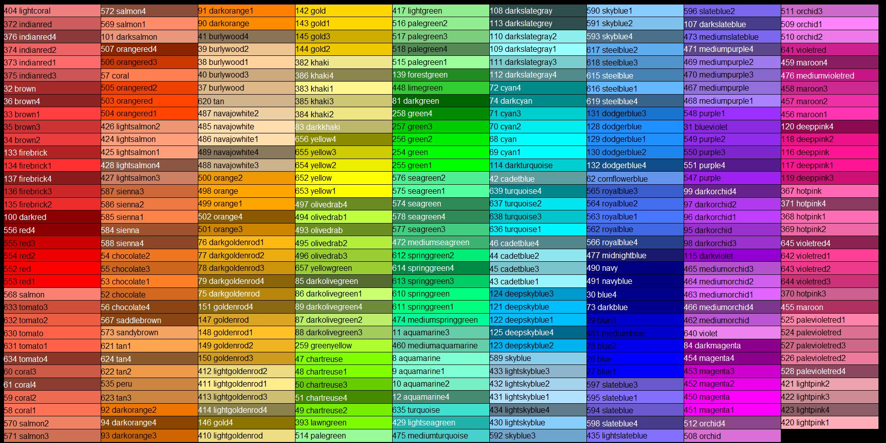
Let us revisit out first scatter plot example:
ggplot(airquality, aes(y = Ozone, x = Temp, color = factor(Month)))
Month has been converted to a categorical variable via factor(Month), consequently discrete colors are expected (at least as many as unique values of Month = 5).
scale_colour_manual(values = c("red","navy","gold","tan","plum"), na.value="gray")
color (or colour) specifies the colors of symbols and all lines in a plot. For bar plots, histograms or filled symbols (pch 21-25) it specifies the border around the filled areas (this is different compared to most base R graphics). The color of areas as bars, confidence bands etc can be specified similarly via scale_fill_manual.
If you don't want to specify the colors by hand. You can use some pre specified color palettes, e.g. scale_colour_brewer(palette = "Set1")
To get an overview which palettes are available use the following code:
library(ggplot2)
library(RColorBrewer)
display.brewer.all()
The color palettes in the middle are called "Qualitative sets". They are especially useful for unordered categorical data (Accent, Dark2, Paired, Pastel1, Pastel2, Set1, Set2, Set3).
All color schemes provided are from the ColorBrewer project:
https://colorbrewer2.org
You sould definitely visit this site, because you can identify schemes with special features, like color-blind friendly or printer friendly sets.
In the example below we would like to produce a scatter plot with different symbols for each month, symbol fill colors according to different levels of wind speed (manully specified colors) and symbol border lines colord according to different levels of solar radiation using a pre specified color-blind friendly palette:
For numeric (continuouse) variables we can specify a gradient from one color to another with:
scale_colour_gradient(low = "green", high = "red")
You have also an alternative function to specify additional colors for the mid level values, e.g. to have the the red, yellow, green traffic light color codes:
scale_colour_gradientn(colors = c("green", "yellow", "red"))
The equivalent of the function scale_colour_brewer for numeric data is scale_colour_distiller.
Compare the two examples below:
Labels & legends
If you have only one legend, it is relatively easy to manipulate it. If you have multiple legends, the fine tuning requires a bit experience. Some legend features are manipulated directly within the scale_... functions, e.g. to change the title of the legend or the labels of the different items) or with the function theme. For instance theme(legend.position = "top") will display the legend on top of the graph whereas 2 numbers between 0 and 1 will place the legend within the plotting area. If you have more than 1 legend legend.direction = "vertical" will arrange the different legends next to each other. In contrast, legend.box = "vertical" will arrange the single items of a legend next to each other.
The labs function is self-explaining. Simply check out the code below:
Finally, you can use:
theme(legend.position="none") to hide the legend.
Axis limits
If you would like to zoom into the plotting area, don't use
scale_y_continuous(ylim = ...
because this throws the data points outside the plotting region away, which is likely not what you want. Instead, use coord_cartesian. Although this has no impact on the individual data points shown, it has an impact on anything calculated from the data, e.g. a regression line or the median for a boxplot.
Themes
ggplot2 has several standard themes. The default theme theme_grey is useful for screens or presentations but not for publications or printing. For publications you would usually choose theme_classic or theme_bw.

themes
You can find additional examples here:
https://ggplot2.tidyverse.org/reference/ggtheme.html
Export
You can export the figures in high quality for publications with the function ggsave. Provide a name for the file and the name of the plot to save it to yout hardsisk. The function uses the file extension to save the plot in the right format. Allowed file extensions include pdf, jpg or tiff. The latter one is the format of choice for many scientific journals. Add always the argument compression = lzw if you export figures as tiff. If you simply save the figure, the figure will be saved with a dimension of 7 x 7 inch which is likly to large. If you change width and height, it may happen that the text is now too large ot too small. play a bit with the arguments height, width, unit, scale, and dpi to get it right, e.g.
ggsave("My_scatter.jpg", p43, width = 7, height = 4, unit = "in", dpi = 300)
Note: the figure above will be saved at 7 x 4 inch at 300 dpi resolution. If you think that text and symbols should be larger: you can modify the figure directly in ggsave, e.g. to increase the size use:
ggsave("My_scatter.jpg", p43 + theme_bw(base_size = 14), width=7, height=4, unit="in", dpi=300)
Now have fun with ggplot2